Welcome to orthopoly’s documentation!#

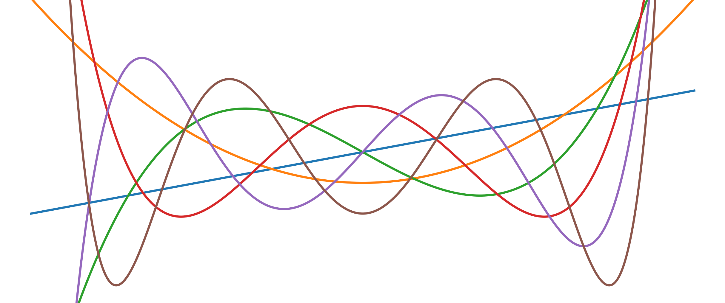
This is a package for using sets of orthogonal functions/polynomials. Currently, it includes Chebyshev, Legendre, and Gegenbauer polynomials. It also has real, two-dimensional spherical harmonics.

Installing/Using#

To install the package, you can

> pip install orthopoly

or you can download/clone the repository, put the top directory in your sys.path, then import it.

chebyshev#

The chebyshev module is pretty well developed. It includes many functions for evaluating the Chebyshev polynomials and their derivatives. The module also includes higher level functions for setting up the elements needed to solve boundary value problems (using the pseudospectral method), interpolate using a Chebyshev grid, and perform the spatial discretization of a PDE solver. Generally, these methods are very well suited to smooth problems.

For performing a discrete Chebyshev transform (generating a Chebyshev expansion from a set of points in 1D), the cheby_coef_setup function can be used. It allows one of the boundary conditions to be the value of the expansion’s first derivative and returns a matrix allowing expansion coefficents to be computed by solving a linear system. When there are no derivatives, the transform can be computed (on the appropriate grid points) with a discrete cosine transform (DCT). The cheby_dct function does this and cheby_dct_setup sets up the grid as well.

Information about the Chebyshev polynomials is widely available, but a few particularly helpful references are below. The Boyd book is especially good.

Boyd, John P. Chebyshev and Fourier spectral methods. Courier Corporation, 2001.
Fornberg, Bengt. A practical guide to pseudospectral methods. Vol. 1. Cambridge university press, 1998.
Canuto, Claudio, et al. Spectral methods. Springer-Verlag, Berlin, 2006.

gegenbauer#

Gegenbauer polynomials \(C_n^m(x)\) are generalizations of Chebyshev and Legendre polynomials. However, chebyshev polynomials of the first kind are implemented by other methods in the chebyshev module, and cannot be computed by the functions in this module.

legendre#

This module implements the Associated Legendre Polynomials, \(P_n^m(x)\), and their first two derivatives in support of the spherical_harmonic module. If \(m=0\), they reduce to the unassociated Legendre polynomials.

spherical_harmonic#

The spherical_harmonic module provides functions for evaluating the real, two-dimensional (surface), orthonormal, spherical harmonics. From the associated Legendre polynomials, the spherical harmonics, their gradients, and their Laplacians can be evaluated. The module also contains some functions for creating grids on the sphere (regular, icosahedral, and Fibonacci) and for creating random spherical harmonic expansions with specific power density relationships (noise). The module does not have functions for performing spherical harmonic analysis (transforming from values on the sphere to expansion coefficients).

For some applications, fitting a spherical harmonic expansion to data in spherical coordinates is useful. A least squares fit can be computed with the pseudoinverse of a matrix full of spherical harmonic function evaluations (see sph_har_matrix and related functions). However, this should only be done when the number of points is much greater than the number of terms in the fitted expansion.

The books cited above have some good discussion of spherical harmonics. Other useful sources include:

Press, William H., et al. Numerical recipes 3rd edition: The art of scientific computing. Cambridge university press, 2007.
Dahlen, F., and Jeroen Tromp. Theoretical global seismology. Princeton university press, 1998.
Bosch, W. “On the computation of derivatives of Legendre functions.” Physics and Chemistry of the Earth, Part A: Solid Earth and Geodesy 25.9-11 (2000): 655-659.